Module 1 — Environments & Agents

All synthetic data projects start with a simulated animal moving through a world. Before working with, for example, head-direction, place, or angular-velocity signals, we need (i.) an Environment: the geometry the animal lives in, and (ii.) an Agent: a motion model that produces rat-like trajectories. This module is about those two objects only: how to build open arenas and 1-D tracks, how RatInABox’s locomotion model works and how to make it move like a real rat, and how to extract clean data from a simulated run.

Agent Movement: A freely-moving rat’s path is not a random walk. Speed and turning are temporally smooth (the animal keeps roughly the same speed and heading for a while, then changes). RatInABox captures this with two separate Ornstein–Uhlenbeck (OU) processes, one on speed and one on rotational velocity, each with a spread and a coherence time (how long it stays correlated). Note the two are shaped differently: in 2D, speed is Rayleigh distributed, so speed_mean sets the Rayleigh scale rather than the mean itself, while rotational velocity is Gaussian. Rodents also hug walls (thigmotaxis).

Outcomes from this Modeule

Create 2-D and 1-D Environment and set scale, aspect, boundary_conditions, and dx
Add walls, holes, and objects to build structured world environments
Create an Agent OU motion model and vary its parameters: (speed_mean, speed_std, speed_coherence_time, etc.)
Learn about the Ag.update() simulation loop and how to inspect live state (Ag.pos, Ag.velocity, Ag.head_direction)
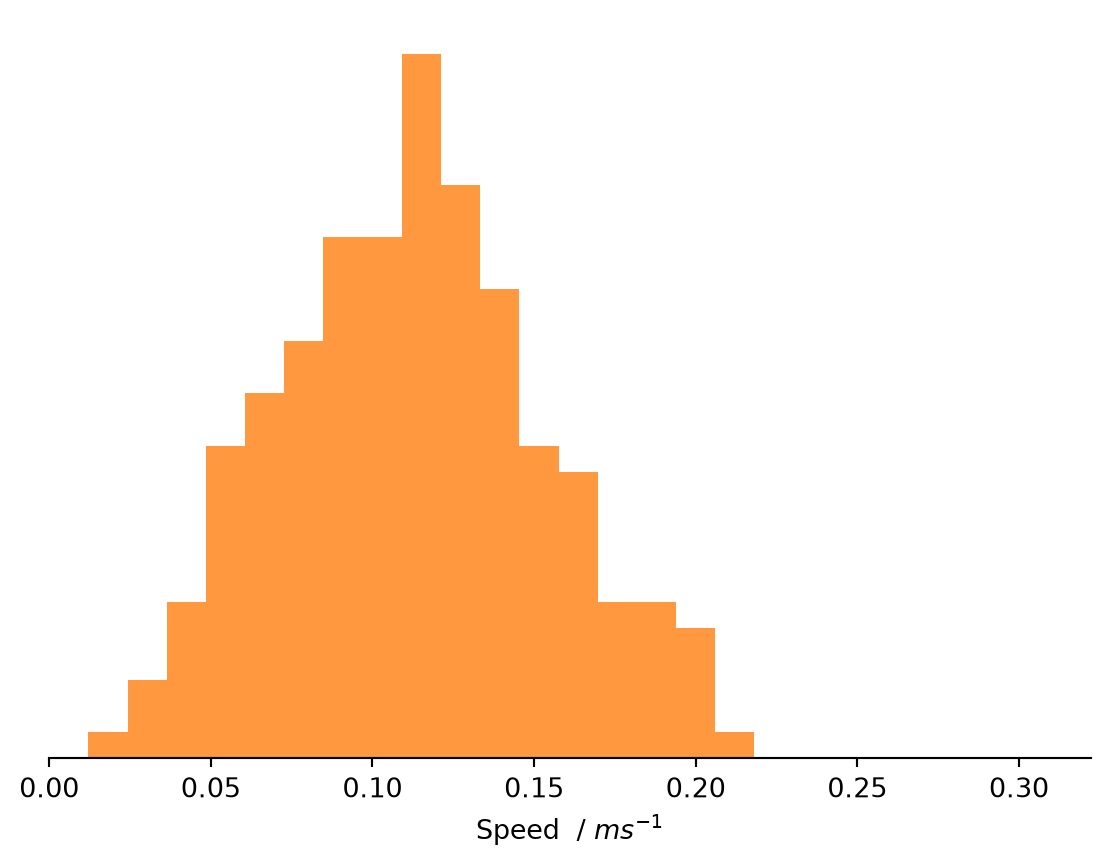
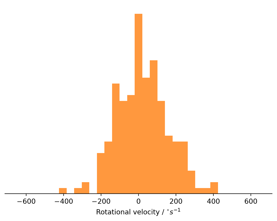
Extract a whole run as arrays with get_history_arrays()
Standard diagnostic plots: trajectory (coloured by time), position heatmap, speed and rotational-velocity histograms
Drive the agent along a known path with import_trajectory, this eventuallycan be used with real trajectory data
How to set Seeds for reproducible runs and science!

Tutorial

0. RiaB Boilerplate

We need to import the correct libraries, disable figure auto-saving, set seeds for both random number generators (RNGs).

import numpy as np
import matplotlib.pyplot as plt
import ratinabox
from ratinabox.Environment import Environment
from ratinabox.Agent import Agent

ratinabox.autosave_plots = False
np.random.seed(0) # for reproducibility
rng = np.random.default_rng(0) # for sampling

Gotcha: ratinabox.stylize_plots() is a function call, not a boolean. Also there is no ratinabox.__version__, instead use import importlib.metadata as md; md.version("ratinabox").

import importlib.metadata as md

print("ratinabox version:", md.version("ratinabox"))
# ratinabox.stylize_plots()   # optional: paper-style plots

ratinabox version: 1.15.3

1. A 2-D environment

The Environment is pure geometry. The most important params are scale (size in metres), aspect (width/height for 2-D), boundary_conditions ("solid" or "periodic"), and dx (the discretisation used later for rate maps).

env = Environment(params={
    "dimensionality": "2D",          # the default
    "scale": 1.0,                    # a 1 m x 1 m box
    "boundary_conditions": "solid",  # walls the animal bounces off
    "dx": 0.01,                      # 1 cm grid for rate maps
})
fig, ax = env.plot_environment()     # returns (fig, ax)
plt.show()

HINT: You can stylize plots to make them look like repo/paper by calling `ratinabox.stylize_plots()`
      This hint will not be shown again

env.plot_environment() draws the box; env.sample_positions(n=100) gives you 100 random valid positions of shape (100, 2), handy for seeding analyses later.

sampled = env.sample_positions(n=100)
print("sample_positions(n=100) ->", sampled.shape)

sample_positions(n=100) -> (100, 2)

2. An Agent and the update loop

The Agent owns the motion model. It is constructed with an environment, and given life by calling Ag.update() repeatedly. Each call advances one dt and appends the new state to the agent’s history.

Ag = Agent(env, params={
    "dt": 0.05,          # 50 ms steps (a default I will be using)
    "speed_mean": 0.08,  # m/s — the OU mean speed (default)
    "speed_std": 0.08,
})

for _ in range(200):     # 200 steps * 0.05 s = 10 s of simulated time
    Ag.update()

Let’s inspect live state:

Ag.pos             # current position, shape (2,)   [ (1,) in 1D ]
Ag.velocity        # current velocity vector, shape (2,)
Ag.head_direction  # current head-direction unit vector, shape (2,)

print("pos            ", Ag.pos, Ag.pos.shape)
print("velocity       ", Ag.velocity, Ag.velocity.shape)
print("head_direction ", Ag.head_direction, Ag.head_direction.shape)

pos             [0.40373176 0.20423275] (2,)
velocity        [0.09661975 0.01397664] (2,)
head_direction  [0.98048365 0.19660065] (2,)

Gotcha: Ag.head_direction is a unit vector, not an angle. But we can recover the heading in radians with np.arctan2(hd[1], hd[0]).

hd = Ag.head_direction
print("|head_direction| =", np.linalg.norm(hd))          # 1.0: unit vector
print("heading =", np.arctan2(hd[1], hd[0]), "rad")

|head_direction| = 1.0
heading = 0.19788969575754342 rad

3. Extracting a run: `get_history_arrays()`

Looking at Ag.pos step-by-step guives us some intuition, but for analysis we want the whole run as arrays. get_history_arrays() returns a dict of formatted numpy arrays for a T-step run:

h = Ag.get_history_arrays()
h["t"]               # (T,)     time in seconds
h["pos"]             # (T, 2)   position
h["vel"]             # (T, 2)   velocity
h["rot_vel"]         # (T,)     ANGULAR velocity
h["head_direction"]  # (T, 2)   unit vectors angle = np.arctan2(hd[:,1], hd[:,0])
h["distance_travelled"]  # (T,)

for key, arr in h.items():
    print(f"{key:20s} {np.asarray(arr).shape}")

t                    (200,)
pos                  (200, 2)
distance_travelled   (200,)
vel                  (200, 2)
rot_vel              (200,)
head_direction       (200, 2)

These types of quantities are what we would use to feed into a model, say an RNN for training. get_history_arrays() is our primary data extraction kickoff. There are a few different flavors of data extraction, but we will encounter those later, for now this is the simplest way to extract.

4. Diagnostic plots

RatInABox comes packaged with diagnostic plots for sanity checks and initial analysis. All return, as expected from a matplotlib-esque API: (fig, ax).

Ag.plot_trajectory(color="changing", colorbar=True)  # path coloured by time
Ag.plot_position_heatmap()                            # occupancy density
Ag.plot_histogram_of_speeds()                         # speed distribution
Ag.plot_histogram_of_rotational_velocities()          # turning distribution
plt.show()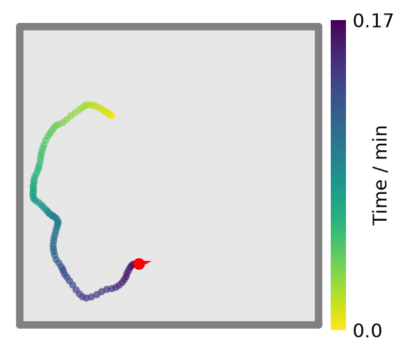

We can also plot the trajectory coloured by time manually if for example we want to build highly custom styled plots.

h = Ag.get_history_arrays()
fig, ax = plt.subplots()
ax.scatter(h["pos"][:, 0], h["pos"][:, 1], c=h["t"], s=4, cmap="viridis")
plt.show()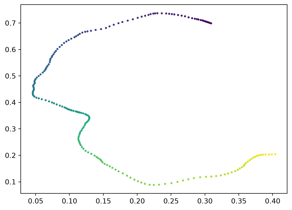

5. Making it move like a rat

speed_mean does not mean what it looks like. In 2D, RatInABox draws speed from a Rayleigh distribution and speed_mean is that distribution’s scale (σ), not its mean. Since the mean of Rayleigh(\(\sigma\)) is \(\sigma \times \sqrt(\pi/2) \approx 1.25 \sigma\), the default speed_mean = 0.08 actually produces a mean speed near 0.10 m/s, at the low end of the 0.1 to 0.2 m/s range that foraging rats cruise at. Note also that speed_std is ignored in 2D (it only does anything in 1D, where speed really is Gaussian with speed_mean as its mean, and setting it to 0 in 2D pins the speed constant). If you want a specific target mean, convert it directly with utils.get_rayleigh_sigma(0.15).

# 10 s is far too short to estimate a mean speed: across seeds that estimate
# ranges from ~0.07 to ~0.15 m/s. Run longer for a stable number.
for _ in range(6000 - 200):          # top up to 6000 steps = 5 minutes
    Ag.update()

h = Ag.get_history_arrays()
empirical_mean_speed = np.linalg.norm(h["vel"], axis=1).mean()

print("speed_mean parameter = 0.08 m/s   (Rayleigh scale, not a mean)")
print(f"predicted mean       = {0.08 * np.sqrt(np.pi / 2):.3f} m/s   (sigma * sqrt(pi/2))")
print(f"empirical mean speed = {empirical_mean_speed:.3f} m/s   (walls + thigmotaxis pull it down)")

speed_mean parameter = 0.08 m/s   (Rayleigh scale, not a mean)
predicted mean       = 0.100 m/s   (sigma * sqrt(pi/2))
empirical mean speed = 0.093 m/s   (walls + thigmotaxis pull it down)

Bump speed_mean and re-measure until the empirical mean lands where you want it. Note the realised mean sits a little below the Rayleigh prediction because walls and thigmotaxis slow the animal, so get_rayleigh_sigma() gets you close but measuring is what confirms it. Other motion knobs worth knowing now:

speed_coherence_time — how long the animal holds a speed (larger = smoother).
rotational_velocity_std — turn sharpness (default 120 * np.pi/180 rad/s, i.e. 120°/s).
thigmotaxis (0–1) — wall-following tendency. Near 1 the animal hugs boundaries; near 0 it roams the interior. This changes where your animal samples space, which changes which place fields get visited. This is a real consideration when generating balanced training data.

6. A 1-D track

Set "dimensionality": "1D" and the environment becomes a line of length scale. Positions are now shape (1,) / (T, 1). This is the world where axis-of-travel tuning lives: an animal running back and forth on a track has only two heading families (leftward vs rightward), which is precisely the structure that elicits axis tuning in subiculum.

env1d = Environment(params={"dimensionality": "1D", "scale": 2.0})  # a 2 m track
Ag1d = Agent(env1d, params={"dt": 0.05})
for _ in range(200):
    Ag1d.update()
h = Ag1d.get_history_arrays()   # h["pos"] has shape (T, 1)

print('1-D h["pos"] shape:', h["pos"].shape)

1-D h["pos"] shape: (200, 1)

/home/runner/work/ratinabox-training/ratinabox-training/.pixi/envs/site/lib/python3.11/site-packages/ratinabox/Agent.py:145: UserWarning: Warning: You have solid 1D boundary conditions and non-zero speed mean.
  warnings.warn(

Gotcha: With a 1-D "solid" boundary and a non-zero speed_mean, RiaB prints a warning (the animal keeps driving into the end walls). This will be resolved when we impose a trajectory next.

7. Driving a known path with `import_trajectory`

Instead of letting the OU model wander, you can hand the agent a trajectory and have it follow. Ag.import_trajectory(times=..., positions=...) loads a (times,) / (times, dim) path and subsequent Ag.update() calls interpolate along it.

env1d = Environment(params={"dimensionality": "1D", "scale": 2.0})
Ag = Agent(env1d, params={"dt": 0.05})

times = np.arange(0, 40, 0.05)
positions = (1.0 + 0.9 * np.sin(2 * np.pi * times / 20.0)).reshape(-1, 1)  # (T, 1)
Ag.import_trajectory(times=times, positions=positions)

for _ in range(len(times)):
    Ag.update()   # now follows the imported path instead of the OU model

Successfully imported dataset from arrays passed
Total of 40.0 s of data available

To confirm it followed, compare the recorded positions against the target path at matching times (interpolate the target onto h["t"] and check the error is tiny).

h = Ag.get_history_arrays()
target_at_t = np.interp(h["t"], times, positions[:, 0])
error = np.abs(h["pos"][:, 0] - target_at_t)

# The loop above ran len(times) steps, so the very last sample sits one dt PAST the end of
# the imported data (times[-1] = 39.95 s) and RiaB extrapolates there.

inside = h["t"] <= times[-1]

fig, ax = plt.subplots(figsize=(8, 3))
ax.plot(times, positions[:, 0], lw=3, alpha=0.35, label="imported path")
ax.plot(h["t"], h["pos"][:, 0], lw=1, color="k", label="agent")
ax.set_xlabel("time (s)")
ax.set_ylabel("position (m)")
ax.legend()
plt.show()

print(f"max |agent - target| inside the imported window = {error[inside].max():.2e} m")
print(f"max |agent - target| including the extrapolated last sample = {error.max():.2e} m")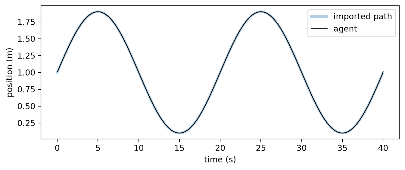

max |agent - target| inside the imported window = 1.11e-15 m
max |agent - target| including the extrapolated last sample = 2.83e-02 m

Key API

Task	Call
2-D world	`Environment(params={"scale":1.0, "aspect":1.0, "boundary_conditions":"solid", "dx":0.01})`
1-D track	`Environment(params={"dimensionality":"1D", "scale":2.0})`
Structure	`env.add_wall([[x0,y0],[x1,y1]])`, `env.add_hole([...])`, `env.add_object([x,y])`
Draw world	`env.plot_environment()` → `(fig, ax)`
Random positions	`env.sample_positions(n=100)` → `(100, 2)`
Agent	`Agent(env, params={"dt":0.05, "speed_mean":..., "thigmotaxis":...})`
Step	`Ag.update()` (loop it)
Live state	`Ag.pos` `(2,)`, `Ag.velocity` `(2,)`, `Ag.head_direction` `(2,)` unit vector
Extract run	`Ag.get_history_arrays()` → `t,pos,vel,rot_vel,head_direction,distance_travelled`
Heading angle	`np.arctan2(hd[:,1], hd[:,0])`
Plots	`Ag.plot_trajectory(color="changing", colorbar=True)`, `Ag.plot_position_heatmap()`, `Ag.plot_histogram_of_speeds()`, `Ag.plot_histogram_of_rotational_velocities()`
Replay a path	`Ag.import_trajectory(times=..., positions=...)` then loop `Ag.update()`
Reproducibility	`np.random.seed(0)` and `rng = np.random.default_rng(0)`

Problems

Problem 1.1

Build a 1 m × 1 m open arena. Simulate 5 minutes at dt=0.05. Plot the trajectory coloured by time.

Show solution 1.1

# 5 minutes at dt = 0.05 s  ->  300 s / 0.05 s = 6000 update() calls.
np.random.seed(0)

env_11 = Environment(params={
    "dimensionality": "2D",
    "scale": 1.0,                    # 1 m x 1 m open arena
    "boundary_conditions": "solid",
    "dx": 0.01,
})
Ag_11 = Agent(env_11, params={"dt": 0.05})

n_steps = int(5 * 60 / 0.05)         # 6000
for _ in range(n_steps):
    Ag_11.update()

h11 = Ag_11.get_history_arrays()

fig, ax = Ag_11.plot_trajectory(color="changing", colorbar=True)
ax.set_title("5 min of foraging in a 1 m x 1 m arena (colour = time)")
plt.show()

print(f"update() calls          : {n_steps}")
print(f'h["pos"] shape          : {h11["pos"].shape}')
print(f"simulated time          : {h11['t'][-1]:.1f} s")
print(f"distance travelled      : {h11['distance_travelled'][-1]:.1f} m")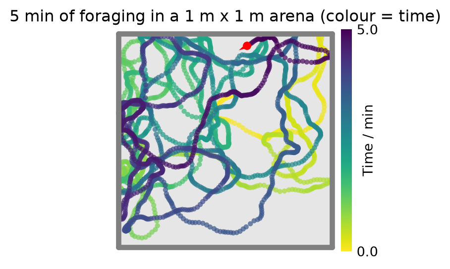

update() calls          : 6000
h["pos"] shape          : (6000, 2)
simulated time          : 300.0 s
distance travelled      : 27.3 m

Problem 1.2

Plot the speed and rotational-velocity histograms. Report the empirical mean speed and then tune the motion parameters so the empirical mean speed is \(\approx\) 0.15 m/s (rat-like) and re-verify. Both speed_mean and speed_std look like they should help. Work out which one actually does in 2D, and explain why.

Show solution 1.2

from ratinabox.utils import get_rayleigh_sigma

env_12 = Environment(params={"scale": 1.0})

def mean_speed_of(sigma, seed=1, n_steps=6000):
    """Run a fresh agent at this speed_mean and return (mean speed, agent)."""
    np.random.seed(seed)
    Ag = Agent(env_12, params={"dt": 0.05, "speed_mean": sigma})
    for _ in range(n_steps):
        Ag.update()
    return np.linalg.norm(Ag.get_history_arrays()["vel"], axis=1).mean(), Ag

# --- BEFORE: the default motion model -------------------------------------------------
speed_before, Ag_slow = mean_speed_of(0.08)

fig, axs = plt.subplots(1, 2, figsize=(9.5, 3.2))
Ag_slow.plot_histogram_of_speeds(fig=fig, ax=axs[0])
Ag_slow.plot_histogram_of_rotational_velocities(fig=fig, ax=axs[1])
axs[0].set_title("speeds (speed_mean = 0.08)")
axs[1].set_title("rotational velocities")
plt.tight_layout(); plt.show()

print(f"BEFORE  speed_mean=0.080  ->  empirical mean speed = {speed_before:.3f} m/s")

# --- WHICH KNOB ACTUALLY MATTERS? -----------------------------------------------------
print("\nDoes speed_std do anything in 2D?")
for std in (0.02, 0.08, 0.40):
    np.random.seed(1)
    A = Agent(env_12, params={"dt": 0.05, "speed_mean": 0.08, "speed_std": std})
    for _ in range(3000):
        A.update()
    m = np.linalg.norm(A.get_history_arrays()["vel"], axis=1).mean()
    print(f"  speed_std = {std:<5} ->  mean speed {m:.4f} m/s")
print("  Identical. In 2D speed is Rayleigh-distributed and `speed_mean` is its SCALE;")
print("  `speed_std` is ignored (except that setting it to 0 pins the speed constant).")
print("  So `speed_mean` is the only knob here. In 1D it would be a different story.")

# --- TUNE: start analytically, then correct for the walls -----------------------------
# E[Rayleigh(sigma)] = sigma*sqrt(pi/2), so get_rayleigh_sigma() inverts that exactly.
# It lands short because walls and thigmotaxis slow the animal, so measure and rescale.
target = 0.15
sigma = get_rayleigh_sigma(target)
print(f"\nAnalytic starting point: get_rayleigh_sigma({target}) = {sigma:.4f}")
for attempt in range(5):
    measured, Ag_fast = mean_speed_of(sigma)
    print(f"  attempt {attempt}: speed_mean={sigma:.4f} -> measured {measured:.4f} m/s")
    if abs(measured - target) < 0.005:
        break
    sigma *= target / measured

# --- AFTER: re-verify ------------------------------------------------------------------
fig, axs = plt.subplots(1, 2, figsize=(9.5, 3.2))
Ag_fast.plot_histogram_of_speeds(fig=fig, ax=axs[0])
Ag_fast.plot_histogram_of_rotational_velocities(fig=fig, ax=axs[1])
axs[0].set_title(f"speeds (tuned speed_mean = {sigma:.3f})")
axs[1].set_title("rotational velocities")
plt.tight_layout(); plt.show()

print(f"\nAFTER   speed_mean={sigma:.4f}  ->  empirical mean speed = {measured:.3f} m/s (target {target})")
print(f"speed-up over the default: {measured / speed_before:.2f}x")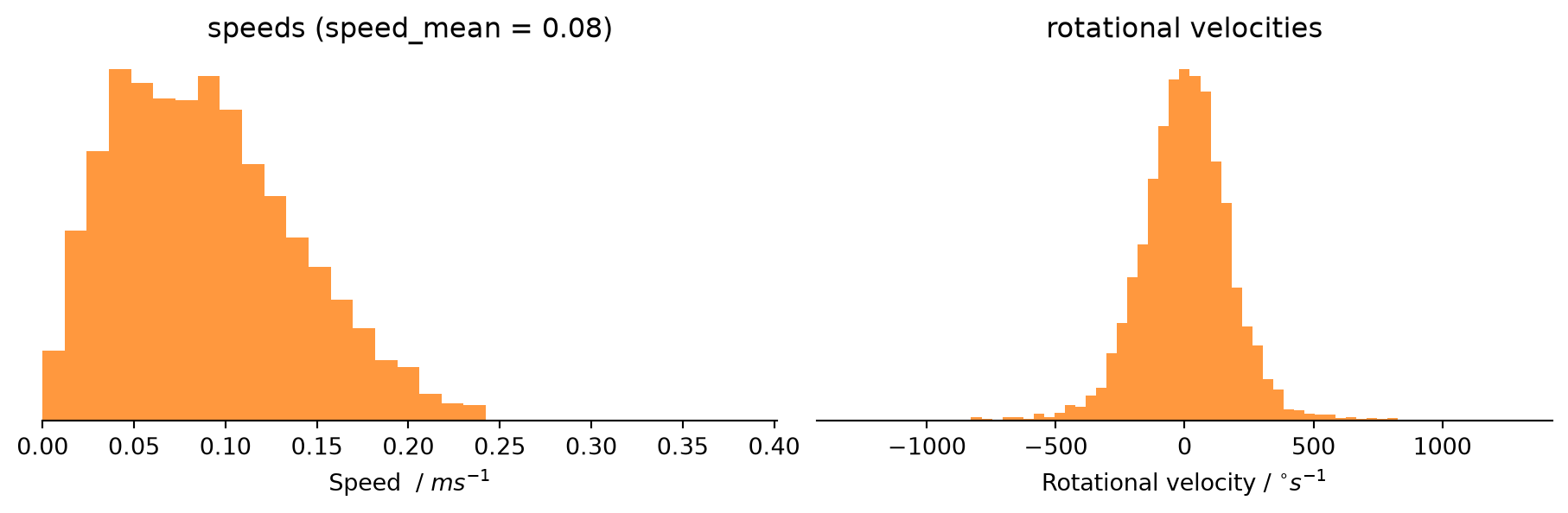

BEFORE  speed_mean=0.080  ->  empirical mean speed = 0.090 m/s

Does speed_std do anything in 2D?
  speed_std = 0.02  ->  mean speed 0.0882 m/s
  speed_std = 0.08  ->  mean speed 0.0882 m/s
  speed_std = 0.4   ->  mean speed 0.0882 m/s
  Identical. In 2D speed is Rayleigh-distributed and `speed_mean` is its SCALE;
  `speed_std` is ignored (except that setting it to 0 pins the speed constant).
  So `speed_mean` is the only knob here. In 1D it would be a different story.

Analytic starting point: get_rayleigh_sigma(0.15) = 0.1197
  attempt 0: speed_mean=0.1197 -> measured 0.1280 m/s
  attempt 1: speed_mean=0.1403 -> measured 0.1581 m/s
  attempt 2: speed_mean=0.1331 -> measured 0.1549 m/s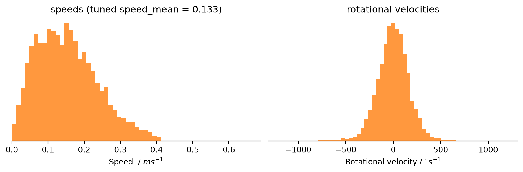


AFTER   speed_mean=0.1331  ->  empirical mean speed = 0.155 m/s (target 0.15)
speed-up over the default: 1.71x

Problem 1.3

Vary thigmotaxis (0.1 vs 0.9). Compare position heatmaps and quantify wall-hugging as the fraction of time spent within 10 cm of any wall.

For a 1 m unit square, distance to the nearest wall is min(x, 1-x, y, 1-y). The two agents are built below, create the heatmaps and the metric.

Show solution 1.3

# Two agents in the same 1 m x 1 m arena, differing ONLY in thigmotaxis.
np.random.seed(2)
env_13 = Environment(params={"scale": 1.0})

agents = {}
for th in (0.1, 0.9):
    A = Agent(env_13, params={"dt": 0.05, "thigmotaxis": th})
    for _ in range(4000):                   # 200 s each
        A.update()
    agents[th] = A

# --- SOLUTION ---
def wall_hug_fraction(agent, margin=0.1, scale=1.0):
    # Fraction of samples within `margin` m of ANY wall of a `scale` m square arena.
    p = agent.get_history_arrays()["pos"]
    d_wall = np.minimum(np.minimum(p[:, 0], scale - p[:, 0]),
                        np.minimum(p[:, 1], scale - p[:, 1]))
    return float((d_wall < margin).mean())

fracs = {th: wall_hug_fraction(A) for th, A in agents.items()}

fig, axs = plt.subplots(1, 2, figsize=(9.5, 4))
for ax, (th, A) in zip(axs, agents.items()):
    A.plot_position_heatmap(fig=fig, ax=ax)
    ax.set_title(f"thigmotaxis = {th}\nwithin 10 cm of a wall: {fracs[th]:.1%} of the time")
plt.tight_layout()
plt.show()

for th, f in fracs.items():
    print(f"thigmotaxis = {th}:  fraction of time within 10 cm of any wall = {f:.3f}")
print(f"the wall-hugging agent spends {fracs[0.9] / fracs[0.1]:.2f}x as long near walls")
print("high thigmotaxis hugs walls more:", bool(fracs[0.9] > fracs[0.1]))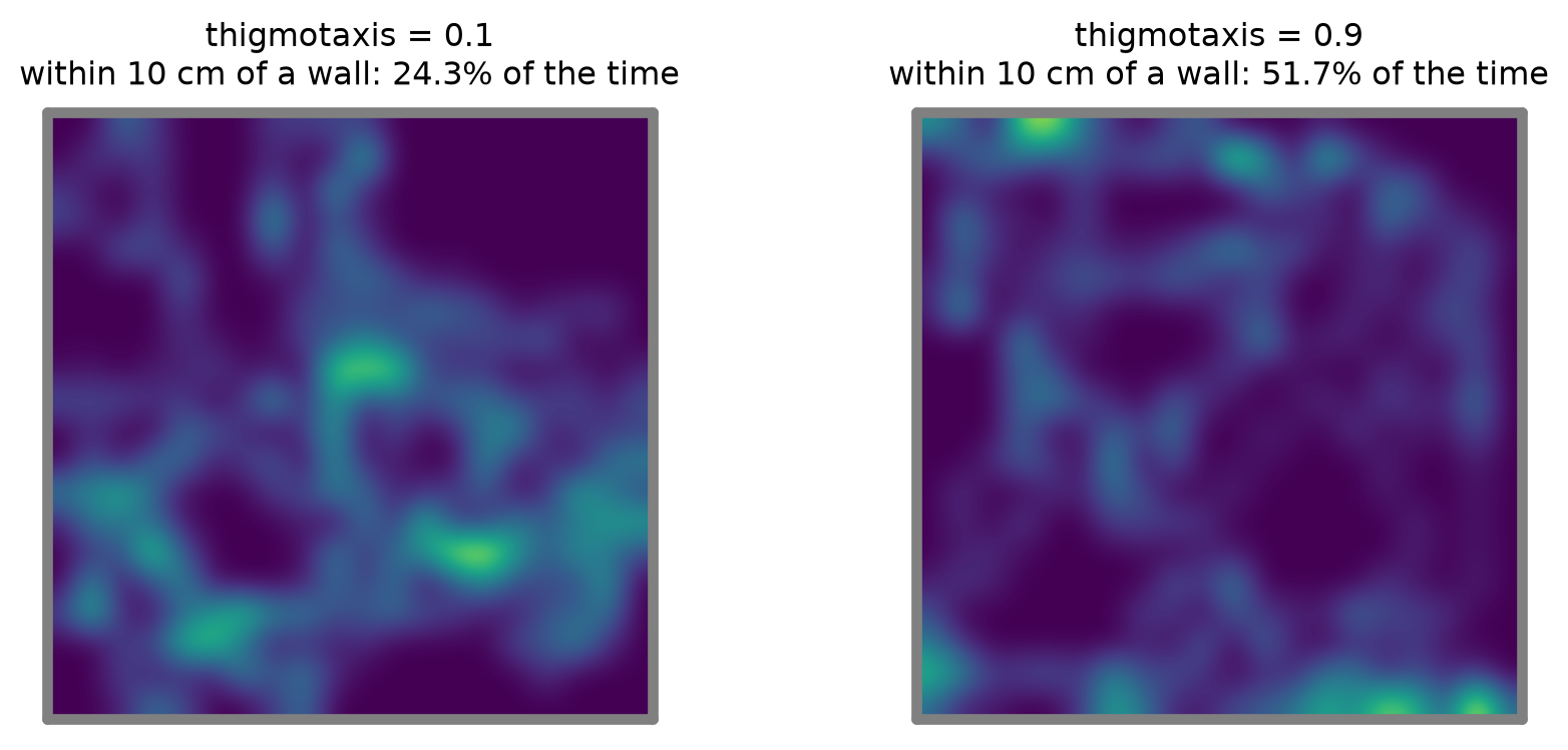

thigmotaxis = 0.1:  fraction of time within 10 cm of any wall = 0.243
thigmotaxis = 0.9:  fraction of time within 10 cm of any wall = 0.517
the wall-hugging agent spends 2.13x as long near walls
high thigmotaxis hugs walls more: True

Problem 1.4

Build a 2 m 1-D track, simulate and plot position vs time.

Remember h["pos"] is now (T, 1), so plot h["pos"][:, 0] against h["t"].

Show solution 1.4

np.random.seed(3)
env_14 = Environment(params={"dimensionality": "1D", "scale": 2.0})   # a 2 m track

# (a) the default agent — note the section-6 Gotcha: with solid 1-D walls and a non-zero
#     speed_mean the animal drives into an end wall and parks there.
Ag_14 = Agent(env_14, params={"dt": 0.05})
for _ in range(3000):                        # 150 s
    Ag_14.update()
h14 = Ag_14.get_history_arrays()

# (b) speed_mean = 0 with a healthy speed_std gives the back-and-forth running that a real
#     linear track produces — this is the world axis-of-travel tuning lives in.
Ag_14b = Agent(env_14, params={"dt": 0.05, "speed_mean": 0.0, "speed_std": 0.2})
for _ in range(3000):
    Ag_14b.update()
h14b = Ag_14b.get_history_arrays()

fig, axs = plt.subplots(2, 1, figsize=(8, 5), sharex=True)
axs[0].plot(h14["t"], h14["pos"][:, 0], lw=1)
axs[0].set_title("default agent (speed_mean = 0.08): drives into an end wall")
axs[1].plot(h14b["t"], h14b["pos"][:, 0], lw=1, color="C1")
axs[1].set_title("speed_mean = 0.0, speed_std = 0.2: back-and-forth running")
axs[1].set_xlabel("time (s)")
for ax in axs:
    ax.set_ylabel("position (m)")
    ax.set_ylim(0, 2)
plt.tight_layout()
plt.show()

print(f'1-D h["pos"] shape        : {h14["pos"].shape}')
print(f"default agent  covers     : "
      f"{h14['pos'][:, 0].min():.2f} - {h14['pos'][:, 0].max():.2f} m of the 2 m track")
print(f"speed_mean=0 agent covers : "
      f"{h14b['pos'][:, 0].min():.2f} - {h14b['pos'][:, 0].max():.2f} m of the 2 m track")

/home/runner/work/ratinabox-training/ratinabox-training/.pixi/envs/site/lib/python3.11/site-packages/ratinabox/Agent.py:145: UserWarning: Warning: You have solid 1D boundary conditions and non-zero speed mean.
  warnings.warn(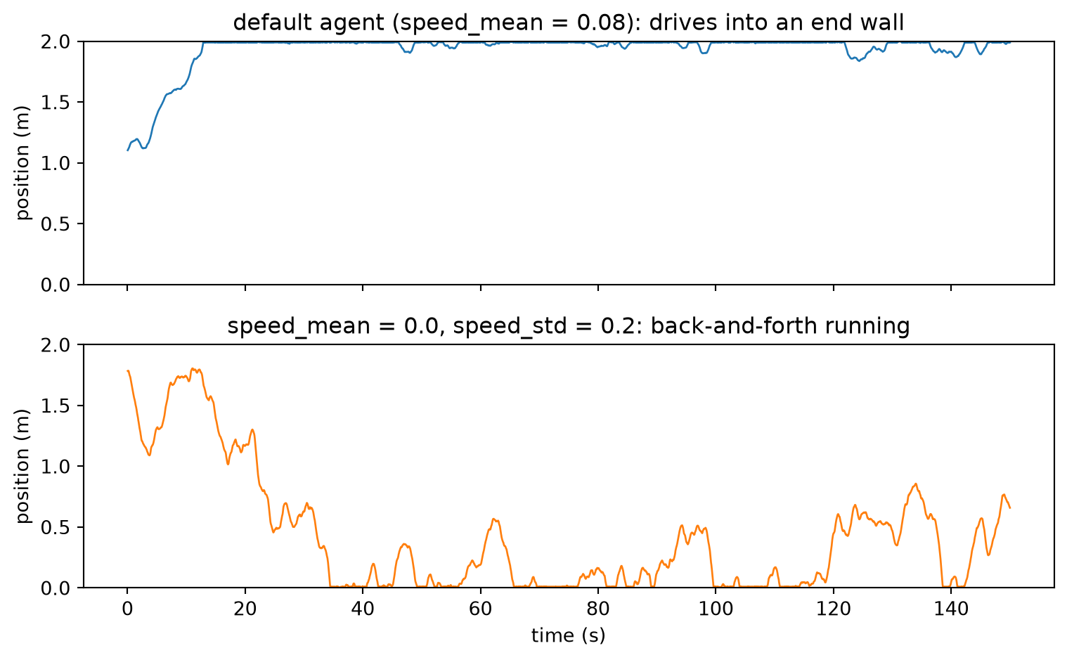

1-D h["pos"] shape        : (3000, 1)
default agent  covers     : 1.10 - 2.00 m of the 2 m track
speed_mean=0 agent covers : 0.00 - 1.81 m of the 2 m track

Problem 1.5

Use import_trajectory to drive the agent along a hand-made back-and-forth path on the 1-D track. confirm it follows.

The track and the clock are given below, but build the (T, 1) position array, import it, loop Ag.update(), and check the error against the target.

Show solution 1.5

# A 2 m 1-D track, a fresh agent, and the clock we want to drive it on.
np.random.seed(4)
env_15 = Environment(params={"dimensionality": "1D", "scale": 2.0})
Ag_15 = Agent(env_15, params={"dt": 0.05})

dt = 0.05
times = np.arange(0, 40, dt)                 # 40 s of hand-made behaviour

# --- SOLUTION ---
# Two laps of 0 -> 2 -> 0, piecewise linear: constant 0.2 m/s runs in each direction.
knot_t = [0.0, 10.0, 20.0, 30.0, 40.0]
knot_x = [0.0,  2.0,  0.0,  2.0,  0.0]
positions_15 = np.interp(times, knot_t, knot_x).reshape(-1, 1)     # (T, 1)

Ag_15.import_trajectory(times=times, positions=positions_15)
for _ in range(len(times)):
    Ag_15.update()                           # follows the imported path, not the OU model

h15 = Ag_15.get_history_arrays()

# Confirm numerically: interpolate the target onto the agent's own timestamps. Only judge
# the samples inside the imported window — the final update() steps one dt past times[-1].
target_at_t = np.interp(h15["t"], times, positions_15[:, 0])
error = np.abs(h15["pos"][:, 0] - target_at_t)
inside = h15["t"] <= times[-1]

fig, ax = plt.subplots(figsize=(8, 3.2))
ax.plot(times, positions_15[:, 0], lw=4, alpha=0.3, label="imported target path")
ax.plot(h15["t"], h15["pos"][:, 0], lw=1, color="k", label="agent (Ag.update())")
ax.set_xlabel("time (s)")
ax.set_ylabel("position (m)")
ax.set_title("import_trajectory: the agent follows the path we handed it")
ax.legend(loc="upper right")
plt.tight_layout()
plt.show()

print(f'imported path shape   : {positions_15.shape}')
print(f'h["pos"] shape        : {h15["pos"].shape}')
print(f"max  |agent - target| : {error[inside].max():.2e} m")
print(f"mean |agent - target| : {error[inside].mean():.2e} m")
print("agent follows the imported path:", bool(error[inside].max() < 1e-6))

Successfully imported dataset from arrays passed
Total of 40.0 s of data available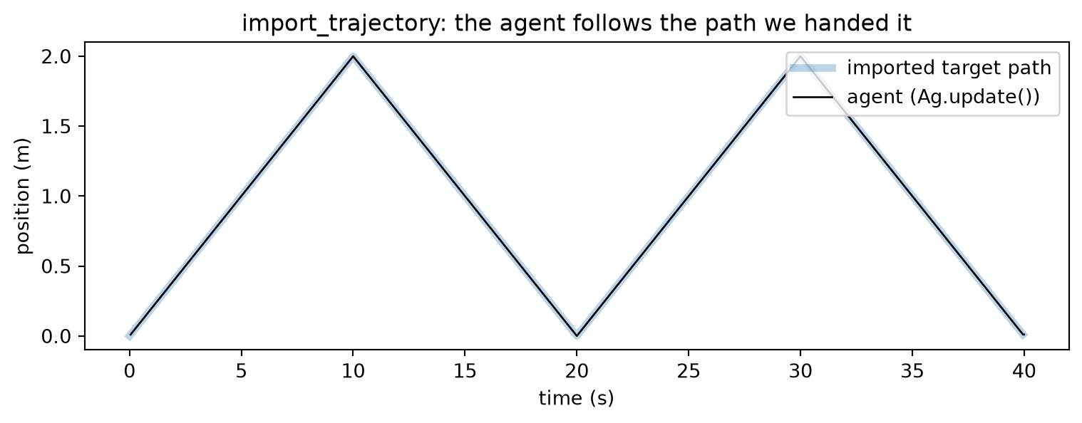

imported path shape   : (800, 1)
h["pos"] shape        : (800, 1)
max  |agent - target| : 5.86e-14 m
mean |agent - target| : 2.80e-16 m
agent follows the imported path: True

References

@article{george2024ratinabox, author = {George, Tom M. and Rastogi, Mehul and de Cothi, William and Clopath, Claudia and Stachenfeld, Kimberly and Barry, Caswell}, title = {{RatInABox}, a toolkit for modelling locomotion and neuronal activity in continuous environments}, journal = {eLife}, volume = {13}, pages = {e85274}, year = {2024}, doi = {10.7554/eLife.85274} }

@article{sargolini2006conjunctive, author = {Sargolini, Francesca and Fyhn, Marianne and Hafting, Torkel and McNaughton, Bruce L. and Witter, Menno P. and Moser, May-Britt and Moser, Edvard I.}, title = {Conjunctive representation of position, direction, and velocity in entorhinal cortex}, journal = {Science}, volume = {312}, number = {5774}, pages = {758–762}, year = {2006}, doi = {10.1126/science.1125572} }